15
Sep 2015
Note on Think Stats Exercise 5.13 Part 1 aka Using what I learnt in a Mathematical Statistics class
NOTE: This post has been delayed by 2 weeks due to me falling sick on the week beginning 23 August. A lot of momentum originally going into the post has been abruptly taken away but heck, I gotta pick up where I left off.
This week I’ve been using my spare time to crack my mind on Think Stats Exercise 5.13 part 1. After skipping Exercise 5.12 because I found it too open-ended and poorly defined for someone who has no experience in mathematical / statistical modelling, I resolved to work on Exercise 5.13 even if the outcome doesn’t seem “good”; well at least I resolved to work on Part 1 of it and I did. And I’m very glad I did. Because I got to use some knowledge I picked up in a Mathematical Statistics class I took in my final semester in university (ST2132 Mathematical Statistics).
NOTE: There is a very high likelihood that I’ve misused some terms due to my rudimentary knowledge in Probability and Statistics. Some of my approaches may also be completely wrong. But I don’t have someone around to guide me and point out my mistakes (as do many many other people), so a lot of what I do is based on my own judgement and intuition.
Source Code
Before we continue, relevant source code is available here as a gist: https://gist.github.com/yanhan/d8fcafdbaa421f0262bf. Most of it is from Think Stats and is licensed under the GNU GPL v3. My code specific to this post is in ch05.py.
The problem
Here is the problem statement:
Suppose that a particular cancer has an incidence of 1 case per thousand people per year. If you follow a particular cohort of 100 people for 10 years, you would expect to see about 1 case. If you saw two cases, that would not be very surprising, but more than two would be rare.
Write a program that simulates a large number of cohorts over a 10 year period and estimates the distribution of total cases.
The “problem solving” process: Questions and Assumptions
Notice that the words problem solving are in quotes, because I don’t think my approach is the only way to look at the problem.
The first thing I asked myself was: Ok. So we gotta do a simulation. But how does one translate 1 case per thousand people per year to a cohort of 100 people for 10 years? I mean, do we just assume that \( P(\text{person gets cancer}) = \frac{1}{1000} \)? Or should this probability be \( \frac{1}{10000} \) since there’s only 100 people for each cohort?
Even more questions:
- Are we assuming independence between the event that person \(A\) contracts cancer and the event that person \(B\) contracting cancer, where person \(A\) and \(B\) are distinct individuals?
- How do we perform the simulation? Do we do assume one of the above probabilities and do it for each person? Do we run the simulation 1 year at a time until we hit 10 years?
So even before we get our hands dirty writing code for the simulation, there are so many things to think about and so many assumptions we have to make.
So I thought for a while and here are my answers to the above questions:
- We indeed assume that \( P(\text{person gets cancer}) = \frac{1}{1000} \), since that’s the assumption given in the question. The confusion about whether \( P(\text{person gets cancer}) \) should vary based on the cohort size we’re looking at and become \( \frac{1}{10000} \) for a cohort of size 100 is a newbie’s mistake. Initially, I couldn’t explain why but while writing this sentence, somehow my mind came up with an explanation that I believe is correct: This confusion is the result of a confusion between the concept of underlying probability vs. the concept of Expectation. Indeed \( P(\text{person gets cancer}) = \frac{1}{1000} \) and once we fix this probability, it will not change regardless of the number of people (very tempted to use the term population here but I’m not sure if it’s the right term) we’re looking at; what will vary when the cohort size changes is the expected number of people who will contract cancer. Case in point: If we look at \(1000\) people and assume that the probability of each one of them getting cancer is \( \frac{1}{1000} \) and any one person getting cancer does not affect whether anyone else gets cancer, then we can model this as a binomial random variable \( X \sim Binom(n = 1000, p = \frac{1}{1000}) \) and the expected number of people getting cancer is given by \( \mathbb{E} = np = 1000 * \frac{1}{1000} = 1 \). However, if we make the same assumptions as before but change the cohort size to \(100\), then the expected number of people getting cancer becomes \( \mathbb{E} = 100 * \frac{1}{1000} = 0.1 \) \ . Man am I glad I wrote this post, just this section alone clarifies a lot of things for me.
- For simplicity, we assume that the event that some person \(A\) contracts cancer is independent of the event that a distinct person \(B\) contracts cancer, regardless of the cohort they are from. In fact, I have no idea how to perform this simulation if we don’t make this assumption.
- We perform the simulation on a per year basis; and for each year, we do it for each cohort; and for each cohort, we do it for each individual. Since we assumed that \( P(\text{person gets cancer}) = \frac{1}{1000} \) and each cohort is modelled as a \( Binom(n = 100, p = \frac{1}{1000}) \) random variable which is just a sum of \( 100 \) i.i.d. \( Ber(\frac{1}{1000}) \) random variables, we can use a CDF inversion algorithm to simulate each \( Ber(\frac{1}{1000}) \) random variable, by generating a \( Unif(0, 1) \) random variable and checking if its probability lies below \( \frac{1}{1000} \). If the value of the \( Unif(0, 1)\) is less than or equal to \( \frac{1}{1000} \), then that person contracts cancer in that year. Because we are tracking the total number of people in a cohort who contracted cancer in a 10 year period, as long as the person contracts cancer in some year, he/she is considered to have contracted cancer in the 10 year period. So to save a little bit of computing time for the simulation, we can effectively ignore that particular person for the rest of the years.
Here’s the code we use to perform the simulation:
# We'll do the simulation 1 year by 1 year
# Each year, about 1 / 1000 people will contract the particular cancer.
# So we assume that for each year, P(person gets cancer) = 1 / 1000
prob_get_cancer = 1.0 / 1000

# Performs a simulation and returns the simulated data
def _perform_simulation(nr_cohorts):
    cohort_size = 100
    nr_years = 10
    simulated_data = []
    # we perform simulation one cohort at a time
    for _ in range(nr_cohorts):
        cancer_cases_in_cohort = 0
        # and for each cohort, we perform the simulation 1 year at a
        # time for `nr_years` years
        for _ in range(nr_years):
            nr_contracted_cancer_in_this_round = 0
            # Once a patient contracts cancer, he/she is counted as a
            # case. Therefore we don't need to perform simulation for
            # that person anymore. The `nr_in_cohort_without_cancer`
            # stores the number of people in the cohort who have not yet
            # contracted cancer (we sound evil here but I don't know how
            # else to put it)
            nr_in_cohort_without_cancer = cohort_size - cancer_cases_in_cohort
            for i in range(nr_in_cohort_without_cancer):
                # this simulates a Ber(p) random variable, where p is
                # the probability of the person contracting cancer
                if random.uniform(0, 1) <= prob_get_cancer:
                    nr_contracted_cancer_in_this_round += 1
            cancer_cases_in_cohort += nr_contracted_cancer_in_this_round
        # we're done simulating the cohort and have the total number of
        # cancer cases in the cohort over 10 years. append it to our
        # data set.
        simulated_data.append(cancer_cases_in_cohort)
    return simulated_data
With that, we perform our simulation by:
nr_cohorts = 1000
simulated_data = _perform_simulation(nr_cohorts)
There’s a reason why we place all our simulation code in a function. We’ll see why later.
The “problem solving” process: Model fitting
Imho, Chapters 3 and 4 of the book have been the most insightful chapters so far, in particular Chapter 4, which introduces the idea of model fitting. Plotting the CDF of a single variable data set (not sure if I’m using the right term here) can offer a lot of insights, especially when you know how to quickly spot some common patterns, or better, fit a lot of commonly used models onto the data. That was exactly what I did.
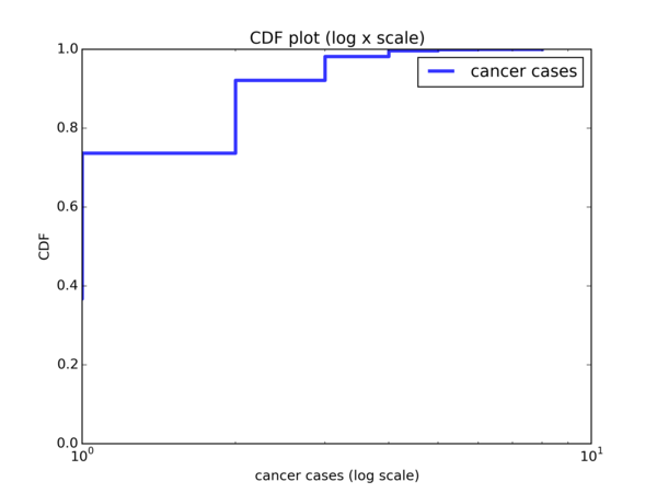
Let’s take a look at the CDF from our simulation data:
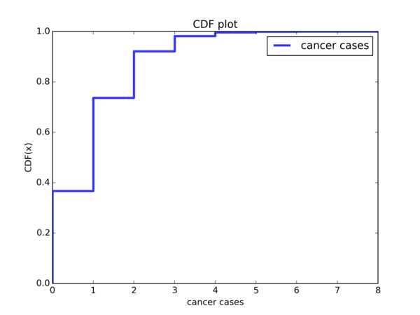
Hmmm ok, so slightly less than 40% of the cohorts have no cancer cases and slightly less than 40% of the cohorts have 1 cancer case. So overall, about slightly less than 80% of the cohorts have 1 or less cancer cases. About 10% to 15% of the cohorts have 2 cancer cases, and less than 10% cohorts see >= 3 cases. So this kind of fits the description given in the book:
If you follow a particular cohort of 100 people for 10 years, you would expect to see about 1 case. If you saw two cases, that would not be very surprising, but more than two would be rare.
And serves as a verification that we are doing our simulation correctly.
Now, let’s transform the CDF in various ways as outlined in Chapter 4 and see if we observe certain trends that reveal to us that the a certain distribution will a good fit for the data.
Trend observation I: the Exponential distribution
The CDF of a random variable from an exponential distribution with parameter λ is given by:
$$ F_{X}(x) = 1 - e^{-λx} \ $$
From Chapter 4.1 of the book, we know that we can perform some transformations and see if we observe a linear trend, first by considering the CCDF (Complementary Cumulative Distribution Function) instead of the CDF:
$$ 1 - F_{X}(x) = e^{-λx} \ $$
So \( 1 - F_{X}(x) \) is the CCDF. We replace it with \( y \):
$$ y = e^{-λx} \ $$
Then take \( log \) on both sides:
$$ \begin{aligned} log(y) &= log(e^{-λx}) \ log(y) &= -λx \end{aligned} $$
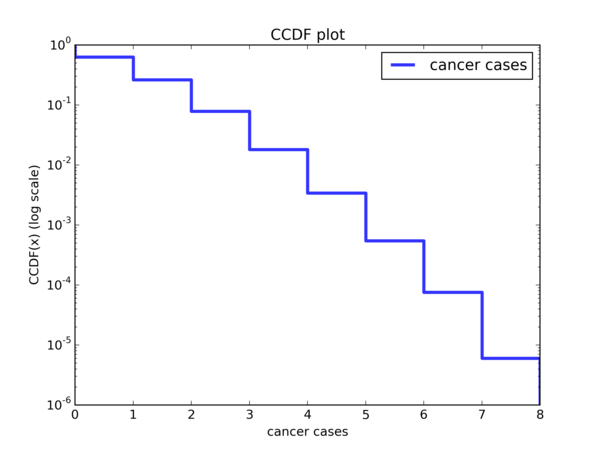
Hence, if we plot \( y = e^{-λx} \) where \( y \) is the CCDF on a \( log\ y \) scale and the exponential distribution happens to be a good model for the data, then we should be observing a linear trend, where \( -λ \) is the gradient of the line. Is that the case? Let’s look at our plot:
Looks like a reasonably linear trend to me. Because I don’t know how to do it using matplotlib, allow me to use Gimp to hand draw a smooth curve:
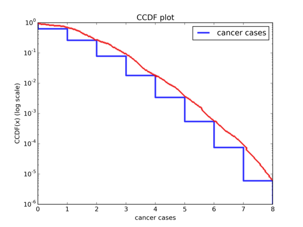
Ok, it wouldn’t be too outrageous to call this linear, or at least very close to it. So the exponential distribution may very well be a good fit. Let’s perform some other transformations on the CDF and see if we can spot other trends.
Trend observation II: the Pareto distribution
Think Stats gives the CDF of the Pareto distribution as follows:
$$ CDF(x) = 1 - (\frac{x}{x_m})^{-\alpha} $$
while the Wikipedia entry for the Pareto Distribution says it is:
$$ CDF(x) = 1 - (\frac{x_m}{x})^{\alpha} $$
There is essentially no difference between the two. For consistency, we shall stick with the form given by Think Stats.
Again, we consider the CCDF of the Pareto Distribution. That is:
$$ 1 - CDF(x) = (\frac{x}{x_m})^{-\alpha} $$
And we replace \( 1 - CDF(x) \) with \( y \) to get:
$$ y = (\frac{x}{x_m})^{-\alpha} $$
Taking \( log \) on both sides:
$$ log(y) = -\alpha log(\frac{x}{x_m}) \ log(y) = -\alpha(log(x) - log(x_m)) \ log(y) = -\alpha log(x) + \alpha log(x_m) $$
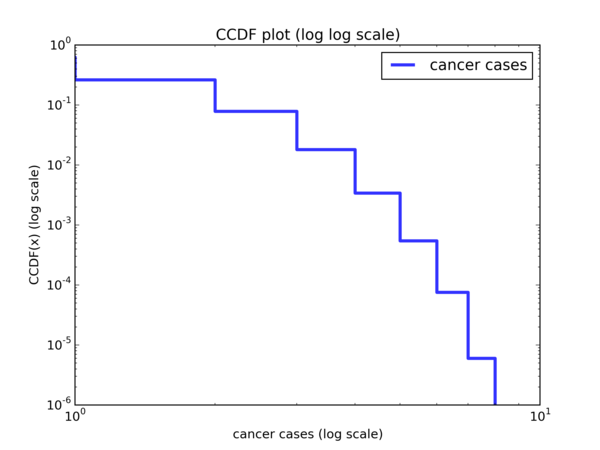
So if we plot the CCDF on a \( log \ log \) scale and the Pareto is a good model for the data, we should see a linear trend with gradient \( -\alpha \) and y-intercept \( \alpha log(x_m) \). Let’s do a \( log \ log \) plot of the CCDF and see if that’s the case:
And with a hand drawn curve:
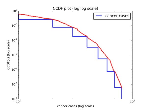
It’s pretty obvious that this is hardly linear. So the Pareto distribution does not seem to be a good model for the data.
Trend observation III: the Log-normal distribution
If we look at the CDF of our simulated data:
We can see that it looks quite different from that of a normal CDF, which looks something like this:
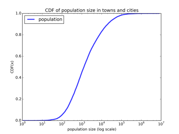
So the normal distribution is not a good fit for our data. But how about the Log-normal distribution? We say that if a random variable \( X \) is log-normally distributed, then \( Y = ln(X) \) has a normal distribution. So if the Log-normal distribution is a good fit for our data, we should see a plot that looks similar to the normal CDF when we plot the CDF on a \( log \ x \) scale. Let’s do the plot:
And… it looks nothing like the CDF of a normal distribution. So the Log-normal distribution is not a good model for our data.
Trend observation IV: the Weibull distribution
The other distribution that we’ve learnt about in Chapter 4, specifically from Exercise 4.6, is the Weibull distribution. Its CDF is given by:
$$ CDF(x) = 1 - e^{-(\frac{x}{λ})^{k}} $$
Again, we consider the CCDF:
$$ 1 - CDF(x) = e^{-(\frac{x}{λ})^{k}} $$
and perform the following manipulations:
$$ 1 - CDF(x) = e^{-(\frac{x}{λ})^{k}} \ log(1 - CDF(x)) = -(\frac{x}{λ})^{k} \ -log(1 - CDF(x)) = (\frac{x}{λ})^{k} \ log(-log(1 - CDF(x))) = k \cdot log(\frac{x}{λ}) \ log(-log(1 - CDF(x))) = k \cdot log(x) - k \cdot log(λ) \ log(log((1 - CDF(x))^{-1})) = k \cdot log(x) - k \cdot log(λ) $$
Admittedly, this is quite a handful. Basically, if we do a \( log \ log \) plot with \( y = log((1 - CDF(x))^{-1}) = log(\frac{1}{1 - CDF(x)}) = log(\frac{1}{CCDF(x)}) \), then we should observe a linear trend with gradient \( k \) and y-intercept \( -k \cdot log(λ) \). Let’s look at the plot:
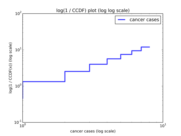
And with a hand drawn curve:
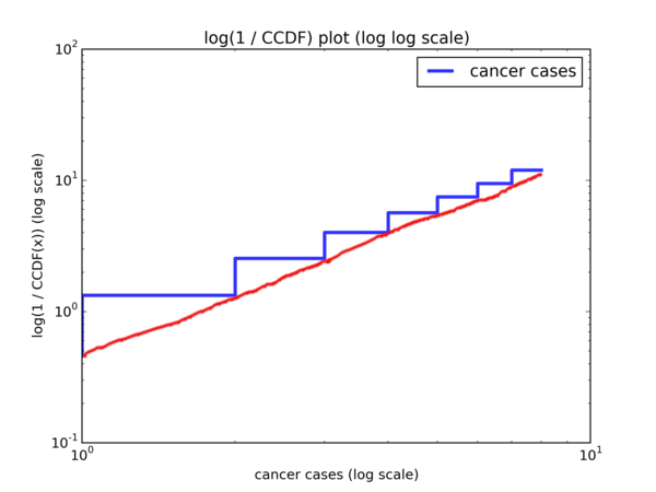
And we indeed observe a linear trend.
Conclusions of Trend Observations
So to recap, we performed various transformations on the CDF to see if any of the Exponential, Pareto, Log-normal or Weibull distributions will be a good model for our data. Based on what we see, it seems that the Exponential and Weibull distributions could be good models for our data. Let’s take a look at the plots again:
Plot of the transform to observe if the Exponential distribution is a good model:
Plot of the transform to observe if the Weibull distribution is a good model:
Now what?
Now that we’ve narrowed down the choices of models to the Exponential and Weibull distributions, what do we do next? It would be to verify if any of them are actually good models. And how do we do that? It seems that we have to find out the concrete Exponential and Weibull distributions that would make for good models. While Think Stats has shown us how to come up with various plots of the CDF of the data and observe if the data can be modelled using some commonly occurring distributions, it doesn’t show us how to do this follow up step, which is to come up with the concrete distributions and see how well they correspond to the CDF.
To make myself clear, let’s say we want to find out the Exponential distribution that would best correspond to our data. We know that the Exponential distribution is parameterized by \( \lambda \). So our job is to find out this appropriate value of \( \lambda \), plot the CDF of the \( Exp(\lambda) \) distribution and compare that against the CDF of our data to see how well they match up. This seems to be a complicated step. Perhaps we should just stop here and call it a day and just move on, after all we did our best and it doesn’t seem that we can do more.
Or is it?
Mathematical Statistics to the rescue
I happen to have taken a Mathematical Statistics class in my final semester of university. ST2132 Mathematical Statistics, to be exact. I didn’t do very well for the class, having gotten a B. The paper was pretty tough and the concepts were pretty abstract for someone whose previous exposure to Statistics was about 3 years ago in a rather poorly taught class. Also, I didn’t see the point to a lot of things I’ve learnt in the class; it all seemed like a bunch of mechanical calculations.
Until I ran into this exercise in the Think Stats book.
For some reason, I recalled that when given a data set that one suspects belongs to some distribution with some unknown parameter(s), one could perform parameter estimation. Ok, I must admit that when I did this exercise, I certainly didn’t think of the term ‘parameter estimation’; it only came up as I was writing this blog post. But I certainly did recall the Method of Moments and Maximum Likelihood Estimate techniques. And I was set.
Model Fitting
Model I: Exponential distribution
So for the Method of Moments method, we take as many moments as necessary, starting from the first moment, and express the moments in terms of the parameters. Then we invert the role of the moments and the parameters and express the parameters in terms of the moments. Finally, we substitute the estimated parameters in place of the actual parameters, and the sample moments in place of the moments. Hopefully we’ll only run into stuff like \( \bar{X} \) which we can easily compute from the data set and have an easier time computing the estimated parameters. The number of such equations we’ll need is equivalent to the number of unknown parameters we need to estimate; sometimes we’ll need to take more moments than unknowns because some moments are equal to \( 0 \), which is useless to us.
Ok, that is quite a mouthful. To be more concrete, suppose we are trying to estimate parameters for a distribution parameterized by \( \alpha \) and \( \beta \). Then there are 3 steps we need to do:
- Take as many moments as necessary and express them in terms of unknown parameters. Suppose we took 2 moments and obtained the following:
$$ \mathbb{E}[X] = \alpha \ \mathbb{E}[X^2] = \frac{1}{\beta} $$
- Express the parameters in terms of the moments.
$$ \alpha = \mathbb{E}[X] \ \beta = \frac{1}{\mathbb{E}[X^2]} $$
- Substitute the estimated parameters in place of the actual parameters, and substitute the sample moments in place of the actual moments. We’ll denote the estimated parameters by placing a caret (or a hat) symbol above how we write the actual parameters, so the estimated parameter for \( \alpha \) will be \( \hat{\alpha} \). For sample moments, the \(k\)th sample moment is defined as \( \frac{1}{n} \displaystyle \sum_{i=1}^{n} X_i^{k} \). So performing the substitution on the above 2 equations:
$$ \hat{\alpha} = \frac{1}{n} \displaystyle \sum_{i=1}^{n} X_i \ \hat{\beta} = \frac{1}{\frac{1}{n} \displaystyle \sum_{i=1}^{n} X_i^2} $$
Let’s see it in action for the Exponential distribution.
The Exponential distribution is parameterized by \( \lambda \), so we only need one equation. Let’s begin by taking the first moment:
$$ \begin{aligned} \mathbb{E}[X] =& \int_{0}^{\infty} x \cdot f(x) dx \ =& \int_{0}^{\infty} x \cdot \lambda e^{- \lambda x} dx \end{aligned} $$
At this point, my limited knowledge of Calculus (which I’m making an effort to pick up) means that it’ll be quite difficult for me to compute this integral. However, there is a trick I’ve learnt from the Mathematical Statistics class, which is that a PDF integrated over its support equals to \( 1 \), and that for certain types of integrals, we can perform some algebraic manipulations to massage the symbols into a PDF that we recognize, barring some constant factors. As long as we can do that and we’re trying to integrate over the same support, then we can simply replace the entire integral with 1.
In this case, the \( x \cdot e^{- \lambda x} \) part of the integral looks like the PDF of a Gamma distribution parameterized by \( \alpha \) (shape) and \( \beta \) (rate), which is \( \frac{\beta ^ \alpha}{\Gamma (\alpha)} x^{\alpha - 1} e^{- \beta x} \), where \( \alpha = 2 \) and \( \beta = \lambda \), barring constant factors. So we pick up from where we left off:
$$ \begin{aligned} \mathbb{E}[X] =& \int_{0}^{\infty} x \cdot \lambda e^{- \lambda x} dx \ =& \ \lambda \cdot \int_{0}^{\infty} x^{2-1} \cdot e^{- \lambda x} dx \ =& \ \lambda \cdot \int_{0}^{\infty} \frac{\lambda^{2}}{\Gamma(2)} x^{2 - 1} \cdot e^{- \lambda x} \cdot \frac{\Gamma(2)}{\lambda^2} dx \ =& \ \lambda \cdot \frac{\Gamma(2)}{\lambda^2} \int_{0}^{\infty} \frac{\lambda^{2}}{\Gamma(2)} x^{2 - 1} \cdot e^{- \lambda x} dx \ =& \ \lambda \cdot \frac{\Gamma(2)}{\lambda^2} \cdot 1 \ =& \ \frac{\Gamma(2)}{\lambda} \ =& \ \frac{(2 - 1)!}{\lambda} \ =& \ \frac{1}{\lambda} \end{aligned} $$
So our first step of taking moments and expressing them in terms of parameters is done. For our next step, we express the parameters in terms of the moments:
$$ \mathbb{E}[X] = \ \frac{1}{\lambda} \ \lambda = \frac{1}{\mathbb{E}[X]} $$
Finally, we substitute the sample moments in place of the actual moments, and substitute the estimated parameter in place of the actual parameter. In other words, we substitute the first sample moment \( \frac{1}{n} \displaystyle \sum_{i = 1}^{n} X_i \) in place of \( \mathbb{E}[X] \), and substitute the estimated parameter \( \hat{\lambda} \) in place of the actual parameter \( \lambda \).
$$ \hat{\lambda} = \frac{1}{\frac{1}{n} \displaystyle \sum_{i=1}^{n}X_i} $$
The first sample moment, \( \frac{1}{n} \sum_{i=1}^{n} X_i \), also written as \( \bar{X} \), can be easily computed from the data set; it is simply the average of the \( X \)’s.
How about the Maximum Likelihood Estimate?
Suppose that the random variables \( X_1, X_2, … , X_n \) have a joint density function \( f(x_1, x_2, … , x_n | \theta) \) for parameter \( \theta \). Then, given observed values \( X_i = x_i \), for \( i = 1, 2, …, n \), the likelihood function of \( \theta \) as a function of \( x_1, x_2, …, x_n \) is given by:
$$ lik(\theta) = f(x_1, x_2, … , x_n | \theta) \ $$
To simplify things, we assume that the \( X_i \)’s are i.i.d. (independently and identically distributed). Then the joint density function can be expressed as a product of the marginal densities. Hence the likelihood function can be written as:
$$ \begin{aligned} lik(\theta) =& f(x_1, x_2, … , x_n | \theta) \ =& \prod_{i=1}^{n} f(X_i | \theta) \end{aligned} $$
So the maximum likelihood estimate of the parameter \( \theta \) is the value that maximizes the likelihood above. That is, it makes the observed data most likely (hence its name).
Often times, it is much easier to maximize the log likelihood instead of the likelihood. Maximizing the likelihood is equivalent to maximizing the log likelihood since log is a monotonic function. Given an i.i.d. sample, the log likelihood is:
$$ \begin{aligned} l(\theta) =& \ log(lik(\theta)) \ =& \ log(\prod_{i=1}^{n} f(X_i | \theta)) \ =& \ log(f(X_1 | \theta) \cdot f(X_2 | \theta) \cdot \ \ldots \ \cdot f(X_n | \theta)) \ =& \ log(f(X_1 | \theta)) + log(f(X_2 | \theta)) \ + \ \ldots \ + \ log(f(X_n | \theta)) \ =& \ \sum_{i=1}^{n} log(f(X_i | \theta)) \end{aligned} $$
To use this for our scenario, suppose \( X_1, X_2, … , X_n \) are i.i.d \( Exp(\lambda) \). Then the log likelihood is given by:
$$ \begin{aligned} l(\lambda ) =& \sum_{i=1}^{n} log(f(X_i | \lambda)) \ =& \sum_{i=1}^{n} log(\lambda e^{- \lambda X_i}) \ =& \sum_{i=1}^{n} [log(\lambda) + log(e^{- \lambda X_i})] \ =& \sum_{i=1}^{n} [log(\lambda) -\lambda X_i ] \ =& \sum_{i=1}^{n} [log(\lambda)] - \sum_{i=1}^{n} [\lambda X_i] \ =& \ n \cdot log(\lambda) - \lambda \sum_{i=1}^{n} X_i \end{aligned} $$
To maximize the log likelihood, we set its first derivative to zero:
$$ \begin{aligned} l’(\lambda) =& \frac{d}{d \lambda} l(\lambda) \ =& \frac{d}{d \lambda} ( n \cdot log(\lambda) - \lambda \sum_{i=1}^{n} X_i ) \ =& \frac{n}{\lambda} - \sum_{i=1}^{n} X_i \ \ 0 =& \ \frac{n}{\lambda} - \sum_{i=1}^{n} X_i \ \frac{n}{\lambda} =& \sum_{i=1}^{n} X_i \ \lambda =& \ \frac{n}{\sum_{i=1}^{n} X_i} \ =& \ \frac{1}{\frac{1}{n} \sum_{i=1}^{n} X_i} \ =& \ \frac{1}{\bar{X}} \end{aligned} $$
Hence, the maximum likelihood estimate of \( \lambda \), which we denote as \( \tilde{\lambda} \), is also \( \frac{1}{\bar{X}} \), which is exactly the same as the method of moments estimate \( \hat{\lambda} \).
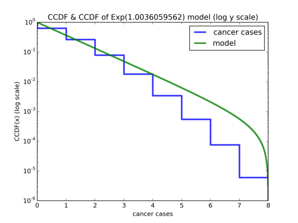
To visually see how well the \( Exp(\hat{\lambda}) \) model is a fit for our data, I came up with 2 plots. First, the plot of the CCDF and the \( Exp(\hat{\lambda}) \) with a similar transform done. Before showing you the plots, here’s the code we use to compute \( \hat{\lambda} \) and draw the Exponential CDF:
# First, we compute lambda = 1 / Xbar
xBar = Mean(simulated_data)
exp_lambda = 1.0 / xBar
# Here, we plot the Exp(lambda) CDF, over increments of 0.01 to make
# it more smooth when we plot it. Otherwise, we'll be getting a plot
# which looks similar to the empirical CDF, which is only defined at
# discrete points.
max_val = max(simulated_data)
exp_lambda_pdf = lambda x: exp_lambda * exp(-exp_lambda * x)
val_to_density = {}
i, incr = 0, 0.01
while i <= max_val:
    val_to_density[i] = exp_lambda_pdf(i)
    i += incr
exp_model_cdf = Cdf.MakeCdfFromDict(val_to_density,
    name="model"
)
Plot for the empirical CCDF and CCDF of our exponential model:
followed by the CDF with the exponential model:
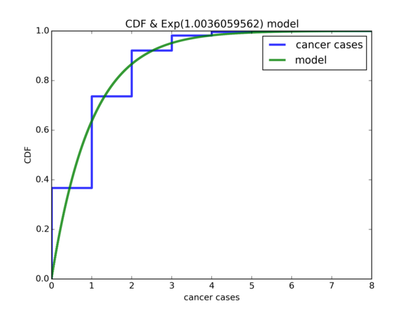
While it is not perfect, other than the fact that the the probability of 0 cancer cases is way off for the model, the rest of the differences are arguably still acceptable. But it seems that we can do better. Suppose that \( X \) is a random variable for the simulated data and \( \mathbb{P}(X <= 0) = p \), so \( p \) is the y-coordinate where \( x = 0 \) for the blue curve and is very close to 0.4 . Suppose \( Y \sim Exp(\hat{\lambda}) \), so the CDF plot of \( Y \) is the green curve. What we want is the value \( y \) such that \( \mathbb{P}(Y <= y) = p \). In other words, the value on the x-axis where the green curve intersects with the blue curve at y-coordinate \( p \). It seems that if we shift the CDF plot of \( Y \sim Exp(\hat{\lambda}) \) by \( y \) units to the left on the x-axis, then the CDF of our model will be a much better fit for the simulated data.
We can obtain \( p \) quite easily, since that is just the fraction of cohorts with zero cancer cases in our simulated data. Once we obtain \( p \), since we know the exact value of \( \hat{\lambda} \), we can perform CDF inversion to get \( y \).
Here is the resulting plot after we shift the Exponential model:
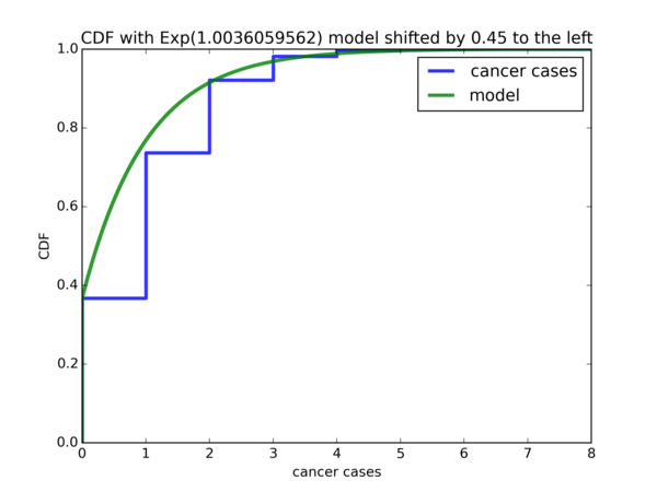
Seems like our modification to the \( Exp(\hat{\lambda}) \) model is a good fit for the data. Let’s move on to our next model, the Weibull distribution.
Model II: Weibull distribution
According to the Wikipedia entry for the Weibull distribution, the PDF of the Weibull distribution is given by \( \frac{k}{\lambda} (\frac{x}{\lambda})^{k-1} e^{-(x / \lambda)^{k}} \). I have to admit that I cheated a bit and looked at the moments for the Weibull distribution and it seems that we’ll need the gamma function, which is defined as \( \Gamma(n) = (n - 1)! \) if \( n \) is a positive integer, or \( \Gamma(t) = \int_{0}^{\infty} x^{t-1} e^{-x} dx \) for complex numbers with a positive real part.
Suppose \( X \sim Weibull(k, \lambda) \). Let us first use the Method of Moments method and take the first moment:
$$ \begin{aligned} \mathbb{E}[X] =& \int_{0}^{\infty} x \cdot f(x) dx \ =& \int_{0}^{\infty} x \cdot \frac{k}{x} (\frac{x}{\lambda})^{k-1} e^{-(x / \lambda)^{k}} dx \ =& \int_{0}^{\infty} k (\frac{x}{\lambda})^{k} e^{-(x / \lambda)^{k}} dx \end{aligned} $$
Now I’m stuck. I decided to perform an integration by substitution. Let \( y = \frac{x}{\lambda} \). Then \( dy = \frac{1}{\lambda} dx \), so \( dx = \lambda dy \). Performing this substitution:
$$ \begin{aligned} \mathbb{E}[X] =& \int_{0}^{\infty} k (\frac{x}{\lambda})^{k} e^{-(x / \lambda)^{k}} dx \ =& \int_{0}^{\infty} k y^k e^{-y^k} \lambda dy \ =& \ \lambda k \int_{0}^{\infty} y^k e^{-y^k} dy \ =& \ \lambda k \int_{0}^{\infty} (y^k)^{2-1} e^{-(y^k)} dy \ =& \ \lambda k \Gamma(2) \ =& \ \lambda k \cdot (2-1)! \ =& \ \lambda k \end{aligned} $$
However, according to Wikipedia, the first moment of a Weibull random variable is \( \lambda \Gamma(1 + \frac{1}{k}) \), which is very different from \( \lambda k \); I mean, in general, it doesn’t seem like \( \Gamma(1 + \frac{1}{k}) = k \) is going to hold. So somewhere along the way, we made a mistake.
After some thinking, I realized that the mistake is here:
$$ \lambda k \int_{0}^{\infty} (y^k)^{2-1} e^{-(y^k)} dy = \ \lambda k \Gamma(2) \ $$
Recall that the Gamma function is defined as \( \Gamma(t) = \int_{0}^{\infty} x^{t-1} e^{-x} dx \). However, notice that in \( \int_{0}^{\infty} ( y^k )^{2-1} e^{-( y^k )} dy \), we are treating \( y^k \) as \( x \), but notice that we are integrating with respect to \( dy \) and not \( dy^k \). If we were integrating with respect to \( dy^k \), then indeed the integral would have evaluated to \( \lambda k \Gamma(2) \).
So it seems like the correct substitution to perform is to let \( y = ( \frac{x}{\lambda} )^k \). Then \( dy = \frac{k}{\lambda} ( \frac{x}{\lambda} )^{k-1} dx \) and \( dx = ( \frac{x}{\lambda} )^{1-k} \cdot \frac{\lambda}{k} dy = y^{\frac{1-k}{k}} \cdot \frac{\lambda}{k} \). Performing the substitutions:
$$ \begin{aligned} \mathbb{E}[X] =& \int_{0}^{\infty} k (\frac{x}{\lambda})^{k} e^{-(x / \lambda)^{k}} dx \ =& \int_{0}^{\infty} k \cdot y \cdot e^{-y} \cdot y^{\frac{1-k}{k}} \cdot \frac{\lambda}{k} dy \ =& \int_{0}^{\infty} \lambda \cdot y^{1 + \frac{1-k}{k}} \cdot e^{-y} dy \ =& \lambda \int_{0}^{\infty} y^{\frac{k+1-k}{k}} \cdot e^{-y} dy \ =& \lambda \int_{0}^{\infty} y^{\frac{1}{k}} e^{-y} dy \ =& \lambda \int_{0}^{\infty} y^{(1 + \frac{1}{k}) - 1} e^{-y} dy \ =& \lambda \Gamma(1 + \frac{1}{k}) \end{aligned} $$
Let us carry on by taking the second moment:
$$ \begin{aligned} \mathbb{E}[X^2] =& \int_{0}^{\infty} x^2 f(x) dx \ =& \int_{0}^{\infty} x^2 \cdot \frac{k}{\lambda} ( \frac{x}{\lambda} )^{k-1} e^{-(x / \lambda)^k} dx \ =& \int_{0}^{\infty} x \cdot k ( \frac{x}{\lambda} )^k e^{-(x / \lambda)^k} dx \end{aligned} $$
Again, we let \( y = ( \frac{x}{\lambda} )^k \), so \( x = \lambda \cdot y^{\frac{1}{k}} \), \( dy = \frac{k}{\lambda} \cdot ( \frac{x}{\lambda} )^{k-1} dx \), \( dx = \frac{\lambda}{k} \cdot ( \frac{x}{\lambda} )^{1-k} dy = \frac{\lambda}{k} \cdot y^{\frac{1-k}{k}} dy \). Performing the necessary substitutions:
$$ \begin{aligned} \mathbb{E}[X^2] =& \int_{0}^{\infty} x \cdot k ( \frac{x}{\lambda} )^k e^{-(x / \lambda)^k} dx \ =& \int_{0}^{\infty} \lambda \cdot y^{\frac{1}{k}} \cdot k \cdot y \cdot e^{-y} \cdot \frac{\lambda}{k} \cdot y^{\frac{1-k}{k}} dy \ =& \int_{0}^{\infty} \lambda^2 y^{\frac{1 + 1 - k}{k} + 1} e^{-y} dy \ =& \ \lambda^2 \int_{0}^{\infty} y^{\frac{2 - k + k}{k}} e^{-y} dy \ =& \ \lambda^2 \int_{0}^{\infty} y^{\frac{2}{k}} e^{-y} dy \ =& \ \lambda^2 \int_{0}^{\infty} y^{(1 + \frac{2}{k}) - 1} e^{-y} dy \ =& \ \lambda^2 \Gamma(1 + \frac{2}{k}) \end{aligned} $$
So we have:
$$ \mathbb{E}[X] = \lambda \Gamma(1 + \frac{1}{k}) \ \mathbb{E}[X^2] = \lambda^2 \Gamma(1 + \frac{2}{k}) $$
Which is not very useful to us, since the parameter \( k \) is stuck inside the gamma function. In fact, the Wikipedia entry for the Weibull distribution states that in general, the \(n\)th moment of a Weibull random variable is given by \( \lambda^n \Gamma(1 + \frac{n}{k}) \). So it doesn’t seem like we’ll be going anywhere by taking additional moments. Time to try the method of Maximum Likelihood Estimate.
Assume that \( X_1, X_2, … X_n \) are i.i.d. \( Weibull(k, \lambda) \), then the joint likelihood is given by \( \displaystyle \prod_{i=1}^{n} f(X_i) = \prod_{i=1}^{n} \frac{k}{\lambda} ( \frac{X_i}{\lambda} )^{k-1} e^{-(X_i / \lambda)^k} \). Maximizing the likelihood is equivalent to maximizing the log likelihood, which is given by:
$$ \begin{aligned} l = log(\prod_{i=1}^{n} f(x_i) ) =& \sum_{i=1}^{n} log(f(X_i)) \ =& \sum_{i=1}^{n} log(\frac{k}{\lambda} ( \frac{X_i}{\lambda} )^{k-1} e^{-(X_i / \lambda)^k} ) \ =& \sum_{i=1}^{n}[ log(\frac{k}{\lambda}) + (k - 1) \cdot log(\frac{X_i}{\lambda}) - ( \frac{X_i}{\lambda} )^k ] \ =& \sum_{i=1}^{n} [ log(k) - log(\lambda) + (k - 1) \cdot log(X_i) - (k-1) \cdot log(\lambda) - ( \frac{X_i}{\lambda} )^k ] \ =& \sum_{i=1}^{n} [ log(k) - k \cdot log(\lambda) + (k-1) \cdot log(X_i) - ( \frac{X_i}{\lambda} )^k ] \ =& \ n \cdot log(k) - nk \cdot log(\lambda) + \sum_{i=1}^{n}[ (k-1) \cdot log(X_i) - ( \frac{X_i}{\lambda} )^k ] \end{aligned} $$
Taking derivatives with respect to \( k \):
$$ \frac{\partial l}{\partial k} = \frac{n}{k} - n \cdot log(\lambda) + \sum_{i=1}^{n} [ log(X_i) - ( \frac{X_i}{\lambda} )^k log(\frac{X_i}{\lambda}) ] \ $$
Taking derivatives with respect to \( \lambda \):
$$ \begin{aligned} \frac{\partial l}{\partial \lambda} =& - \frac{nk}{\lambda} + \sum_{i=1}^{n} [ -(-k) \frac{X_i^k}{\lambda^{k+1}} ] \ =& - \frac{nk}{\lambda} + k \cdot \sum_{i=1}^{n} \frac{X_i^k}{\lambda^{k+1}} \ =& - \frac{nk}{\lambda} + \frac{k}{\lambda^{k+1}} \cdot \sum_{i=1}^{n}X_i^k \end{aligned} $$
Setting \( \frac{\partial l}{\partial \lambda} = 0 \):
$$ -\frac{nk}{\lambda} + \frac{k}{\lambda^{k+1}} \cdot \sum_{i=1}^{n} X_i^k = 0 \ \frac{nk}{\lambda} = \frac{k}{\lambda^{k+1}} \cdot \sum_{i=1}^{n} X_i^k \ \frac{\lambda^{k+1}}{\lambda} = \frac{k}{nk} \cdot \sum_{i=1}^{n} X_i^k \ \lambda^k = \frac{1}{n} \sum_{i=1}^{n} X_i^k $$
Setting \( \frac{\partial l}{\partial k} = 0 \):
$$ \frac{n}{k} - n \cdot log(\lambda) + \sum_{i=1}^{n} [ log(X_i) - ( \frac{X_i}{\lambda} )^k \cdot log(\frac{X_i}{\lambda}) ] = 0 \ \frac{n}{k} - n \cdot log(\lambda) + \sum_{i=1}^{n} [ log(X_i) - ( \frac{X_i}{\lambda} )^k \cdot log(X_i) + ( \frac{X_i}{\lambda} )^k \cdot log(\lambda) ] = 0 \ \frac{n}{k} - n \cdot log(\lambda) + \sum_{i=1}^{n} [ log(X_i) ] - \frac{1}{\lambda^k} \cdot \sum_{i=1}^{n} [ X_i^k \cdot log(X_i) ] + \frac{log(\lambda)}{\lambda^k} \sum_{i=1}^{n} [X_i^k] = 0 \ \frac{n}{k} - \frac{1}{\lambda^k} \sum_{i=1}^{n} [ X_i^k \cdot log(X_i) ] + \frac{log(\lambda)}{\lambda^k} \sum_{i=1}^{n} [ X_i^k ] = n \cdot log(\lambda) - \sum_{i=1}^{n} [ log(X_i) ] \ $$
Substituting \( \lambda^k = \frac{1}{n} \sum_{i=1}^{n} X_i^k \):
$$ \frac{n}{k} - \frac{1}{\lambda^k} \sum_{i=1}^{n} [ X_i^k \cdot log(X_i) ] + \frac{log(\lambda)}{\lambda^k} \sum_{i=1}^{n} [ X_i^k ] = n \cdot log(\lambda) - \sum_{i=1}^{n} [ log(X_i) ] \ \frac{n}{k} - \frac{1}{\frac{1}{n} \sum_{i=1}^{n} [ X_i^k ] } \sum_{i=1}^{n} [ X_i^k \cdot log(X_i) ] + \frac{log(\lambda)}{\frac{1}{n} \sum_{i=1}^{n} [ X_i^k ]} \sum_{i=1}^{n} [ X_i^k ] = n \cdot log(\lambda) - \sum_{i=1}^{n} [ log(X_i) ] \ \frac{n}{k} - \frac{\sum_{i=1}^{n} [ X_i^k \cdot log(X_i) ]}{\frac{1}{n} \sum_{i=1}^{n} [ X_i^k ]} + \frac{log(\lambda)}{\frac{1}{n}} = n \cdot log(\lambda) - \sum_{i=1}^{n} [ log(X_i) ] \ \frac{n}{k} - \frac{n \cdot \sum_{i=1}^{n} [ X_i^k \cdot log(X_i) ]}{\sum_{i=1}^{n} [ X_i^k ]} + n \cdot log(\lambda) = n \cdot log(\lambda) - \sum_{i=1}^{n} [ log(X_i) ] \ \frac{n}{k} - \frac{n \cdot \sum_{i=1}^{n} [ X_i^k \cdot log(X_i) ]}{\sum_{i=1}^{n} [ X_i^k ]} = - \sum_{i=1}^{n} [ log(X_i) ] \ \frac{n}{k} = \frac{n \cdot \sum_{i=1}^{n} [ X_i^k \cdot log(X_i) ]}{\sum_{i=1}^{n} [ X_i^k ]} - \sum_{i=1}^{n} [ log(X_i) ] \ k^{-1} = \frac{\sum_{i=1}^{n} [ X_i^k \cdot log(X_i) ]}{\sum_{i=1}^{n} [ X_i^k ]} - \frac{1}{n} \sum_{i=1}^{n} [ log(X_i) ] \ k = ( \frac{\sum_{i=1}^{n} [ X_i^k \cdot log(X_i) ]}{\sum_{i=1}^{n} [ X_i^k ]} - \frac{1}{n} \sum_{i=1}^{n} [ log(X_i) ] )^{-1} \ $$
So now we have these 2 equations: \( \lambda^k = \frac{1}{n} \sum_{i=1}^{n} X_i^k \) and \( k = ( \frac{ \sum_{1}^{n} X_i^k \cdot log(X_i) }{ \sum_{1}^{n} X_i^k } - \frac{1}{n} \sum_{i=1}^{n} [ log(X_i) ] )^{-1} \), and we see that the one for \( \lambda^k \) depends on the value of \( k \), whereas the one for \( k \) does not depend on \( \lambda \), but is expressed in terms of itself and… I don’t know how to solve it. Typically, this is where things are glossed over during a Mathematical Statistics class, where students are told that “oh, you can solve the equation for \( k \) using a statistical software package”, but aren’t actually shown how to do it.
I did remember such situations happening in ST2132 (the Mathematical Statistics class I’ve taken), where we were trying to maximize the log likelihood for i.i.d. \( X_1, … X_n \) and the underlying distribution is one which is quite well studied. And we ran into this situation and the the lecturer and the notes mentioned that these are non-linear equations which will be quite difficult to evaluate by hand and can be solved numerically using a statistical software package.
I was trying to do this in Python, after all that is the language that Think Stats uses. So I googled a bit and read some questions and answers on Stack Overflow that seemed to be doing what I wanted. But I wasn’t sure, after all I was pretty new to all these and know absolutely nothing about it. I remembered I have a friend doing a PhD in Operations Research at MIT who might be familiar with these things. So I asked him for a bit of help which he kindly rendered.
Perhaps it was luck and persistence that got me through. I guess it was the query “python solve numerical equation” that yielded what I needed. Namely, this answer on Stack Overflow by CT Zhu and this answer on Stack Overflow by nibot. It seemed to me that one of scipy.optimize.root or scipy.optimize.fsolve was what I needed. Since the answer by CT Zhu and nibot both made use of scipy.optimize.fsolve and there was code there, I decided to go ahead with scipy.optimize.fsolve.
Documentation for scipy.optimize.fsolve states that it:
Returns the roots of the (non-linear) equations defined by
func(x) = 0given a starting estimate.
Notice that we have
$$ k = ( \frac{ \sum_{i=1}^{n} [ X_i^k \cdot log(X_i)] }{ \sum_{i=1}^{n} [ X_i^k ] } - \frac{1}{n} \sum_{i=1}^{n} [ log(X_i) ] )^{-1} $$
So in order to make use of scipy.optimize.fsolve, we have to convert it to a function equal to \( 0 \). That is simply \( ( \frac{ \sum_{1}^{n} [ X_i^k \cdot log(X_i)] }{ \sum_{1}^{n} [ X_i^k ] } - \frac{1}{n} \sum_{1}^{n} [ log(X_i) ] )^{-1} - k = 0 \) .
And how about the initial estimate? nibot’s answer states the following helpful tip:
A good way to find such an initial guess is to just plot the expression and look for the zero crossing.
So I did just that:
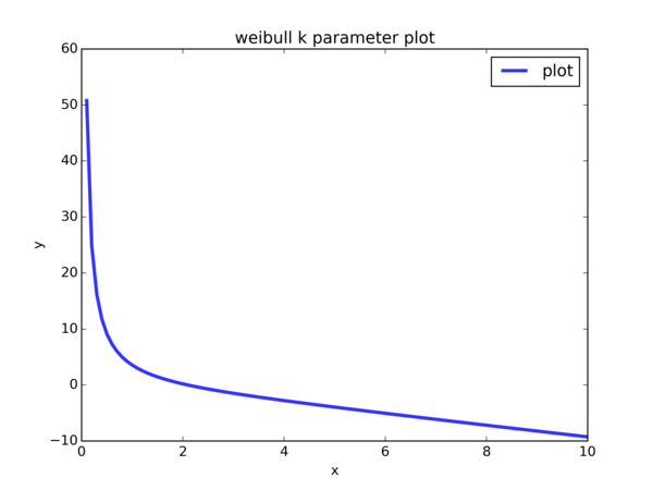
Values of \( x \) are supplied to the equation \( f(k) = ( \frac{ \sum_{1}^{n} [ X_i^k \cdot log(X_i)] }{ \sum_{1}^{n} [ X_i^k ] } - \frac{1}{n} \sum_{1}^{n} [ log(X_i) ] )^{-1} - k \) (so \( k \) takes on each value of \( x \) ’s we are plotting). We see that the curve intersects with the line \( y = 0 \) at approximately \( x = 2 \). So \( 2.0 \) is an ok initial guess to supply to scipy.optimize.fsolve.
Notice that in \( f(k) = ( \frac{ \sum_{1}^{n} [ X_i^k \cdot log(X_i)] }{ \sum_{1}^{n} [ X_i^k ] } - \frac{1}{n} \sum_{1}^{n} [ log(X_i) ] )^{-1} - k \), there is \( log(X_i) \). For our simulated data, a large number of cohorts have 0 cancer cases, so \( X_i = 0 \) for those \( i \). However, \( log \) is undefined at \( 0 \). Hence, we have to exclude those data points during parameter estimation.
Here’s the code for parameter estimation of \( k \) using the method of Maximum Likelihood Estimate:
X_without_zero = list(filter(lambda x: x > 0, simulated_data))
X_without_zero_len = len(X_without_zero)
log_X_without_zero = [log(x) for x in X_without_zero]
one_over_n_sum_of_log_X_without_zero = \
    sum(log_X_without_zero) / float(X_without_zero_len)
# equation we're trying to find roots
def _eqn_for_k(k):
    numer = 0.0
    for i in range(X_without_zero_len):
        numer += (X_without_zero[i] ** k) * (log_X_without_zero[i])
    denom = 0.0
    for i in range(X_without_zero_len):
        denom += (X_without_zero[i] ** k)
    return 1.0 / (numer / denom - one_over_n_sum_of_log_X_without_zero) - k

# This is a rough estimate from looking at the k parameter plot
initial_guess = 2.0
weibull_model_shape = scipy.optimize.fsolve(_eqn_for_k,
    [initial_guess]
)[0]
And once we obtain the MLE for \( k \), we can easily compute the MLE for \( \lambda \). Since \( \lambda^k = \frac{1}{n} \sum_{i=1}^{n} X_i^k \), then \( \lambda = ( \frac{1}{n} \sum_{i=1}^{n} X_i^k )^{ \frac{1}{k} } \). The question is, since we excluded the zero data points when computing the MLE for \( k \), should we also exclude those points when computing the MLE for \( \lambda \)? Frankly speaking, I do not know. So I computed one value of \( \lambda \) that uses the zero data points and another one that excludes them:
weibull_model_scale_on_full_data = (
    sum((x ** weibull_model_shape for x in simulated_data)) / \
        float(nr_cohorts)
) ** (1.0 / weibull_model_shape)
weibull_model_scale_on_non_zero_data = (
    sum((x ** weibull_model_shape for x in X_without_zero)) / \
        float(X_without_zero_len)
) ** (1.0 / weibull_model_shape)
From this point, we’re going to use \( \hat{\lambda} \) to denote the value of \( \lambda \) that is computed using the full data set, and we’re going to use \( \widetilde{\lambda} \) to denote the value of \( \lambda \) that is computed using the non-zero values in the data set.
We’re going to do some plots. We’ll be needing the PDF of the Weibull, defined as \( f(x) = \frac{k}{\lambda} ( \frac{x}{\lambda} )^{k-1} e^{-(x / \lambda)^k} \) for \( x \geqslant 0 \). In code:
def _weibull_pdf(shape, scale, x):
    return (shape / scale * (x / scale) ** (shape - 1) *
        exp(-((x / scale) ** shape))
This next part makes use of a for loop to do some plots for the 2 values of \( \lambda \):
for scale, root_suffix in [
    (weibull_model_scale_on_full_data, "scale-on-full-data",),
    (weibull_model_scale_on_non_zero_data, "scale-on-non-zero-data",),
]:
First, I did a CDF plot of the simulated data along with the Weibull model:
weibull_val_to_density = {}
i, incr, max_val = 0, 0.01, max(simulated_data)
while i <= max_val:
    weibull_val_to_density[i] = _weibull_pdf(
        weibull_model_shape, scale, i
    )
    i += incr
weibull_model_cdf = Cdf.MakeCdfFromDict(weibull_val_to_density,
    name="model"
)
myplot.Cdfs([empirical_cdf, weibull_model_cdf])
myplot.Save(
    root="ex5-13-p1-cdf-with-weibull-model-{}".format(
        root_suffix
    ),
    formats=["pdf", "png",],
    xlabel="cancer cases",
    ylabel="CDF(x)",
    title="CDF & Weibull model",
)
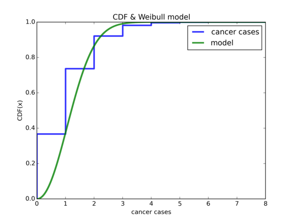
Plot of empirical CDF and \( Weibull(\hat{\lambda}, k) \) CDF:
Plot of empirical CDF and \( Weibull(\widetilde{\lambda}, k) \) CDF:
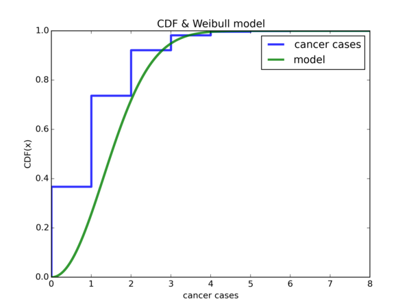
If we let \( W \) denote either one of our Weibull random variable, notice that \( \mathbb{P}(W <= 0) \approx 0 \). However, it is about \( 0.4 \) for the empirical CDF. It also seems that if we shift the Weibull CDF plot to the left by 1 unit in the x-axis, then either model will be much better for our data, that is, if we ignore the region from \( [-1, 0) \). Let’s do it:
weibull_val_minus_one_to_density = dict(
    map(lambda x: (x[0] - 1, x[1]),
        weibull_val_to_density.items()
    )
)
weibull_model_minus_one_cdf = Cdf.MakeCdfFromDict(
    weibull_val_minus_one_to_density, name="model"
)
Plot of empirical CDF and \( Weibull(\hat{\lambda}, k) \) CDF shifted by -1 unit along the x-axis:
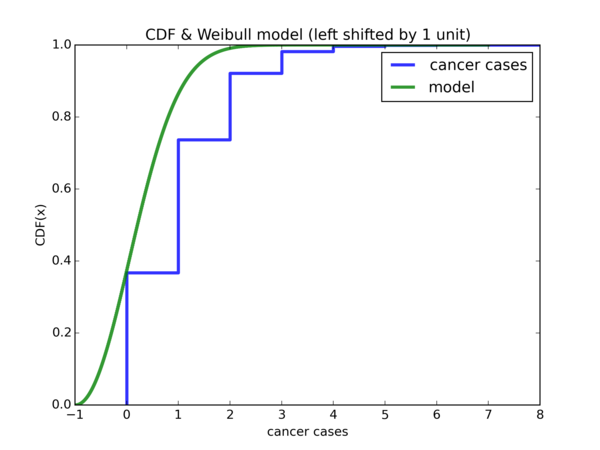
Plot of empirical CDF and \( Weibull(\widetilde{\lambda}, k) \) CDF shifted by -1 unit along the x-axis:
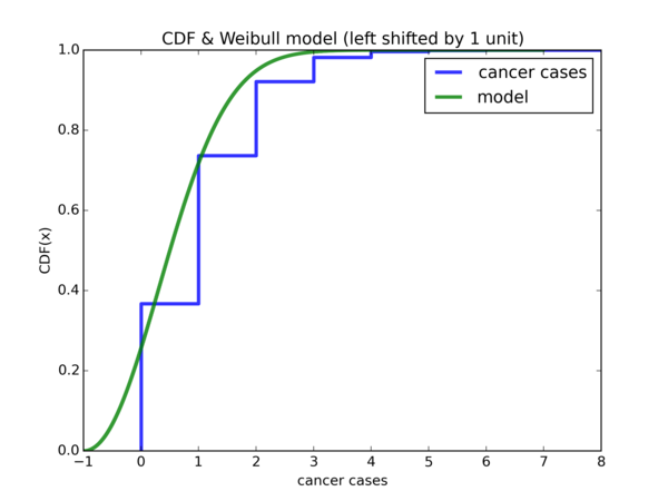
Hmm, despite some discrepancies, that indeed is the case. Let us take it a step further and accumulate all the densities from \( [-1, 0) \) and put them under \( 0 \) and leave the rest of the densities as they are:
sum_of_negative_and_zero_density = sum(
    map(lambda y: y[1],
        filter(lambda x: x[0] <= 0,
            weibull_val_minus_one_to_density.items()
        )
    )
)
weibull_val_to_density = dict(
    filter(lambda x: x[0] > 0,
        weibull_val_minus_one_to_density.items()
    )
)
weibull_val_to_density[0] = sum_of_negative_and_zero_density
weibull_model_negative_grouped_with_zero_cdf = Cdf.MakeCdfFromDict(
    weibull_val_to_density, name="model"
)
Resulting plot for \( Weibull(\hat{\lambda}, k) \):
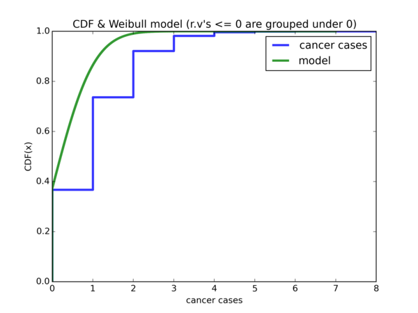
Resulting plot for \( Weibull(\widetilde{\lambda}, k) \):
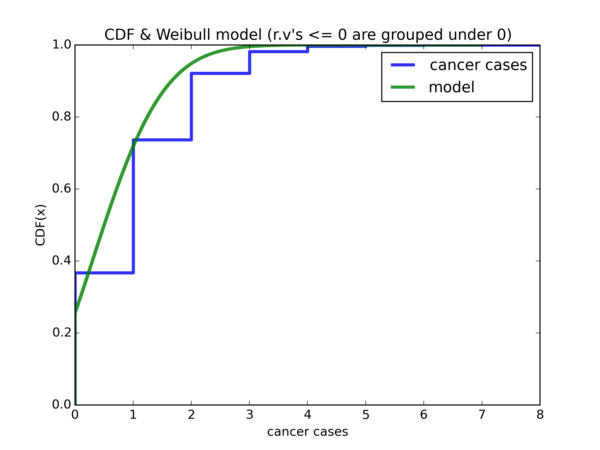
So \( \hat{\lambda} \) offers a good start for \( x = 0 \), but using \( \widetilde{\lambda} \) is a lot better for \( x = 1 \) onwards.
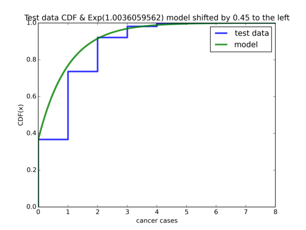
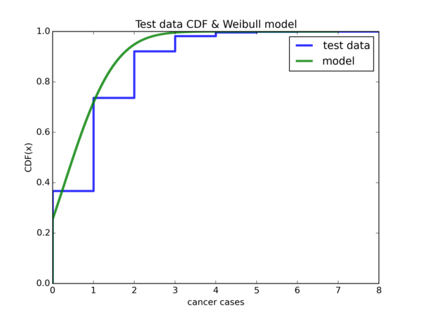
Validating our models
We’ve done model fitting using the Exponential and Weibull distributions. The question is, how well do they generalize? Let’s perform another simulation to find out (and this is where our _perform_simulation function really shines):
test_data = _perform_simulation(nr_cohorts)
test_data_cdf = Cdf.MakeCdfFromList(test_data, name="test data")
Exponential model:
\(Weibull(\hat{\lambda}, k) \) model:
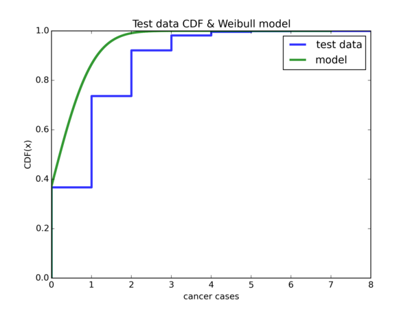
\(Weibull(\widetilde{\lambda}, k) \) model:
I think there are much more mathematically rigorous ways to assess the strength of our models, but I don’t know them well and at this point, I feel that I’ve spent too much time and effort writing this blog post (it took me much longer to write this post than work on the actual problem).
Conclusion
There are probably a lot of things that can be done better. These are the ones that I know of:
- Using proper stopping rules to determine the number of cohorts we should use for the simulation, instead of using an arbitrary number like \( 1000000 \) as I did
- Using more rigorous ways to determine how well our models fare on other simulated data sets
- I did something crazy by shifting the model based on the Exponential distribution to the left by accumulating densities, and the same trick was used for the model based on the Weibull distribution. I have to confess that for this step, mathematically I have no idea whether what I’m doing is valid and how we can characterize the resulting distribution.
- During parameter estimation of \( k \) for the Weibull model, I discarded all the \( X_i = 0 \) values. Later on, I didn’t know whether to use the entire simulated data set or the same truncated data set that we used for paramter estimation of \( k \) to estimate \( \lambda \).
I learnt a lot from thinking a bit more about this exercise and wondering:
- Can we do more than just doing the various variants of the CDF plots and observing trends?
- What is the next step that we can do?
- Should we try to plot the distributions we’re using as models and see visually how well they fit the data?
- What will enable us to plot such distributions?
Then I realized that I have some familiarity with the Exponential and Normal distributions, and while the Pareto and Weibull distributions are new to me, I did a small blog post on the Pareto Distribution and also an exercise on the Weibull distribution so they are not entirely unfamiliar to me. I went on to realize that these distributions are are defined by parameters. For instance, the Exponential distribution is parameterized by \( \lambda \), while the Normal distribution is parameterized by its mean \( \mu \) and variance \( \sigma^2 \).
Probably because of the preparation I did for the final exam of the ST2132 Mathematical Statistics class I took earlier this year, I recalled that there are ways in which we can figure out the parameters given a data set that we know (or in this case, believe) comes from a certain distribution - namely the Method of Moments and Maximum Likelihood Estimate method. This gave me the possibility to explore the exercise on a deeper level instead of just stopping at the step where we look at the various variants of the CDF plots to see if they display some trend. Taking action on this newfound knowledge was the next very crucial step.
While some people may think that it’s a waste of time to derive the algebraic form of the Method of Moments and MLE parameter estimates of the various distributions by hand, especially when the results are available on the Internet, I think that this is a very good revision of the Statistics that I’ve picked up earlier this year. In particular, it was a very interesting exercise to figure out the parameter estimates for the Weibull distribution - not just because I figured out a really bad Calculus mistake I made along the way, but also because it forced me to figure out which libraries to use to solve for an equation \( f(x) = 0 \) numerically - just so I could come up with a model based on the Weibull distribution.
After doing all that work, I figured that it would be great it I could blog about it - it was a terrific decision. Some of the benefits I’ve gained out of writing this blog post:
- Writing this blog post clarified a lot of things for me, because whenever I’m trying to explain something that I don’t fully understand, I’m forced to spend time to think through what exactly I’m trying to explain, after all I can’t just write some incoherent junk. This leads to a much greater understanding and solidification of the knowledge I’ve picked up compared to if I was to just do the exercise and call it a day. Some examples of what I’ve spent time figuring out are:
- Expectation vs. Probability (yes, I know I’m a noob to even confuse them)
- Why we can use Bernoulli random variables to simulate whether each individual in a cohort contracts cancer
- Greater confidence that we’re doing the simulation correctly
- That the Method of Moments and the method of Maximum Likelihood Estimate are used for parameter estimation. I was using them in the Python code without realizing I was doing parameter estimation - it only occurred to me when I was writing this post. It is my belief that knowing the name of something makes a difference.
- Somewhere in the middle of writing this post, I decided to make the source code available as well. As such, I was forced to clean up a lot of the code I wrote, which was in a rather messy state. It’s still somewhat messy after the cleanup but a lot better than before the cleanup.
- A combination of 1. making mistakes in the code 2. refactoring the code 3. making changes to the code so it does new things meant that I had to regenerate the various plots. Many many times. Initially, the code generated the plots in EPS and PDF format. Each time I had to regenerate the plots, I would open up the PDF file, take a screenshot, crop it, then copy and paste it to the images folder for the blog. It was very tedious. Add on to the fact that there were some plots on which I manually drew a curve in red ink using Gimp. After several times, I got sick of doing everything manually. There was nothing I could do about the part where I had to draw a curve manually for some of the plots (thankfully there were not a lot of those and I could delay this process to after everything else was done), but the process by which I had to obtain the final images of the plots for this post was annoying me greatly. So I wondered: can I generate images of the plots instead of just EPS and PDF? Like, PNG images. Turns out that matplotlib can generate plots in PNG format. Next thing on my mind was: ok, is there a way I can programmatically resize the plots so I don’t have to manually crop them anymore? There’s a way to do that as well, using ImageMagick. And I can write a shell script to resize all the images using ImageMagick, dumping the output of each resize to a destination image in the blog’s images folder. All by running 2 commands, one for the python code to generate the plots, the other to do the image resizing. Automation at its finest.
- For
scipy.optimize.fsolve, we need to specify an initial guess. Initially, I supplied \( 1.0 \) probably because \( 0 \) didn’t work. I didn’t actually know the use of the initial guess and essentially filled in a number just because I had to fill in something, until I read nibot’s answer and thought that it would be a good idea to plot a curve of the \( k \) parameter and see where it crosses the \( y = 0 \) line. Visual inspection of the plot determined that \( 2.0 \) will be a closer estimate to the parameter than \( 1.0 \). So I changed my code to use that. Through this process, I obtained a much better understanding of the purpose of the initial guess inscipy.optimize.fsolve. I don’t know if this is true (but I’m thinking that it is), I also read behzad.nouri’s answer which says that no numerical algorithm can figure out all the solutions. I assume I have to add this: “especially if the initial guess is way off”.
There might be more stuff I’ve left out but these are probably the most important ones.
This is also the second rather long blog post I’ve written since my first real blog post (if you don’t count the “Hello World!” blog post), A very long AngularJS tutorial. And it’s slightly more than 2 years since then. This blog post is a lot more obscure than the AngularJS tutorial and is a purely academic exercise that is probably of interest only to myself, but the sense of accomplishment that I feel for completing this post is much greater than that for the AngularJS tutorial, especially because I feel that the topic of this post, Mathematical Statistics, is harder than AngularJS. And unlike the last time, I’m no longer a student and I did this during my spare time outside working hours - that means a lot to me because it is a demonstration that I had the discipline to pull through. I hope to author more posts of this nature (a longer and more involved nature) in the future on some topic in Mathematics, Statistics or Machine Learning - preferrably all of them at the same time =P I hope I’m not biting off more than I can chew (again).
To greater knowledge!
Credits
Ng Yee Sian, for providing assistance.
References
- python - Function returns a vector, how to minimize in via Numpy (answer by CT Zhu)
- Solve an equation using a python numerical solver in numpy (answer by nibot)
- Solve an equation using a python numerical solver in numpy (answer by behzad.nouri)
- scipy.optimize.root - SciPy v0.13.0 Reference Guide
- scipy.optimize.fsolve - SciPy v0.13.0 Reference Guide
Disclaimer: Opinions expressed on this blog are solely my own and do not express the views or opinions of my employer(s), past or present.